For Some Likes
After 2 hours
After 20 minutes
-------------------------------------------
Farming Simulator 17 SEEDS AND FERTILIZER #4 - Duration: 18:04.
HI GUYS !!!! Welcome to Farming Simulator 17 Mods Channel This is the fourth episode of the series SEEDS AND FERTILIZER. In this video I show you some new mods you can use to plant and fertilize your fields.
JOHN DEERE 8030 SERIES Front Attacher 5 Engine Setup 3 Wheel Setup 4 Design Setup
IC CONTROL SPACE Illuminated Dash
Amazone EDX 6000 TC 6m Working Width Crops: maize, sugar beet, soya beans, sunflower
Vss Front Cultivator 5m Working Width Colorable
Seed Express 1260 Semi Trailer Fillable only with seeds, fertilizer and potatos. 45,000l Capacity Colorable
Upgraded Seed and fertilizer storage Placeable Silos
Changelog: Removing grass improves when placing, Fertilizer bearing bug fixes Shovel triggered with seed Fill particles New silo for better removal
Seed Express 1260 Semi Trailer Open Cover And Ladders X KEY Pipe Out O KEY
This is game stock KVERNELAND OPTIMA V Sowing Machine is not compatible :p
I made some mistakes in this video but I decided to share it with you to give you some advice what to AVOID
1) Most of the time game stock tools are not compatible with modded tools.
2) If you adapt more than one implement on your tractor the option HIRE WORKER It is likely to malfunction
3) If you decide to combine Front cultivator and sowing machine try to have the same working width or if you can not find the same working width Sowing Machine must be wider.
My first thought to combine Vss Front Cultivator and Amazone EDX 6000 TC ...
But my the calculations were wrong and I made the wrong choice to use game stock KVERNELAND OPTIMA V Sowing Machine
So the Front Cultivator it was wider and a part of the field stay unplanted
To overload the sowing machine , must be stop and folded
the worker confused
If you enjoy watching my videos... Give thumb up SUBSCRIBE FOR MORE And for any question ( or just for say HI!!) LET comment I will be happy to answer you...... bb
-------------------------------------------
Amazing Street Wall Painting Art Competition In Lahore Held By Master Paints - Duration: 11:58.
Amazing Street Wall Painting Art Competition In Lahore
Sponser By Master Paints
Along Maulana Shaukat Ali Road University Side Wall
More Then 100 Paintings By More Then 500 Artist
Watch Full Video To Give Balanced Review Through Comment Box
-------------------------------------------
EOS s2: Tag Team PVP BG!~ - Duration: 3:12.
Welcome! ʕ•ᴥ•ʔ
♥Lucystar + RenGasai Tag Team ♥
Save yourself Lucy!! ◉_◉
Time for a ninja kill!
Ninja kill 2! ☠
Double sided tag team ftw!
Thank you for watching! ❤
-------------------------------------------
CSGO-Funny Moments #1 Russian Team - Duration: 3:14. For more infomation >> CSGO-Funny Moments #1 Russian Team - Duration: 3:14.
 -------------------------------------------
19. Physics | MOD | Graphical Analysis of Motion | by Ashish Arora (GA) - Duration: 17:11.
Dear students, now we are going to use graphical analysis of motion. as we are studying rectilinear
motion, in rectilinear motion 3 types of graph are used in motion analysis. we'll see that
these graphs are quite helpful, in solving various kind of problems of , rectilinear
motion also. these three types of graph are . displacement versus time graph. second is,
velocity versus time graph . and the third is, acceleration versus time graph. we also
discuss the variant of displacement time graph as, distance time graph . we'll also discuss
distance versus time graph. we'll also discuss speed versus time graph, because , some particular
type of problems are also asked on distance and speed versus time graphs. but we don't
need to spend much time on these at, slight variations of displacement and velocity time
curves. lets discuss these one by one. now if we talk about displacement versus time
graphs . these are also known as , position versus time graphs. there is no difference
between position versus time and displacement versus time graphs. say for a given rectilinear
motion, we, draw the displacement time curve, like this. so this is the curve, according
to which, the position of a particle varies with time. so its function is given as x=
f of t. in this situation at any instant of time, (t) we can directly get the position
of particle by using, this curve, or by substituting the value of time in this function. say if
this point is p, we draw a tangent , of this curve at this point p, and say it makes an
angle theta with the time axis so we can simply state. the slope of the curve. at point p
can be written as, d x by d t, which is = tan theta . and we all know that d x by d t, can
be directly written as, instantaneous velocity of the particle at this position p. so by,
displacement time graph , at any point if we want to calculate , or we want to evaluate
the instantaneous velocity of the particle, we just need to find out the slope of the
curve, at that point and the slope will be directly give us the, instantaneous velocity
of the particle at that point. so in this situation we can see that, this tangent makes
an acute angle, with the, time axis, here we can simply state the velocity v p which
is tan theta , will be a positive , quantity. if we talk about the decreasing part of the
curve at a point q, if we consider a tangent, you can state, this angle theta dash will
be an obtuse angle. so at point q, the instantaneous velocity can be written as tan theta dash.
and tangent of the obtuse angle can be written as, a negative physical quantity. so in the
decreasing part of curve we can say with time the displacement is coming down , or displacement
is decreasing. or, as if we talk about the position of particle it is moving towards
origin. so we can state vector ally the velocity will be, negative. we can also talk about
various situations, like, for a practical situation . if say, a particle moves, in such
a way, that, first it accelerates, than it moves uniformly, and then say it retards . initially
say it was at rest, and finally also say it'll come to rest . so first it accelerates its
velocity increases, than it moves uniformly , and then finally, it comes to rest. now
in such situations, if particle is accelerating we can simply state the slope will first increase.
and then it moves uniformly that mean its slope remains constant, because you can see
the slope is giving as the instantaneous velocity. and if it it retards, that mean the slope
decreases and finally it becomes zero. so if we draw, the displacement time graph, of
such a motion, we can state first slope is increasing, the curve goes like this you can
see , continual sly the angle which , tangent makes with the time axis increasing. and then
say, for a time t 1 it is, accelerating, and from time t 1 to t 2 or you can say for a
duration t 2 , it moves uniformly so we can draw a straight line. so here, the whole slope,
for the duration t 2 remains constant, then it retards , so you can simply draw a curve
like this. which for another duration say t 3. now in this situation finally you can
see the slope become zero and earlier also slope was zero. this is the curve , which
is representing a motion where particle first accelerate, then moves uniformly and then,
retards . similar to this if we just, consider an experimental
situation like, say this positive direction of x axis. from origin a particle starts.
it moves with a velocity v. it goes up to a particular position in a time t 1. then
for a time t 2 it remains at rest over there , and then it comes back to origin, with the
same velocity v. in a time t 3. so from zero to t 1, it was moving uniformly , up to, this
position, say we write maximum displacement x m. for a duration t 2 it remains at rest,
and then , for at time t 2 it'll start, moving in opposite direction, and time t 3 it comes
back. now if we draw, the , position versus time graph, for this motion. you can simply
state it t = 0 particle starts, with an uniform velocity, uniform velocity means the slope
remains constant here we can write tan theta = v. this was the time t 1 for which the particle
was moving uniformly. then you can state up to time t 2 , or for the duration t 2 minus
t 1 it remains at rest. so its position remains constant i.e. at, x m. and then, it'll start
coming back so the velocity, is in opposite direction or we can say, when it was moving
toward (right) velocity was positive and now velocity is negative. so it comes down and
at a time t 3 it'll reach the, original position back. so, you can simple state again x becomes
zero. and say this angle is theta dash, so we can again write tan theta dash is equals
to v. now this angle will be , 180 minus theta, and we can state the, tangent of obtuse angle
is negative . so this angle theta dash can be directly taken as the angle by which we
can directly calculate the negative slope . so this is the, curve which is drawn , for
uniform motion then rest for some duration , and then again uniform motion in opposite
direction . now if similar , this is the curve which we call as position time curve or position
time graph . if similar graph is drawn for distance time .
let us draw distance time graph for the same, motion of particle when it is moving then
rest , taking rest and then coming back. so you can simply state , if we talk about displacement
, it first increases to x m then decreases to zero. but when we talk about distance , we
can state distance is continually increasing, because from here to here the distance is
x m, and when it comes back , the total distance travelled by the particle will become 2 x
m. now only difference in position time and distance time graph, can be taken, that, distance
time graph , if this is taken as distance, distance time graph will never come down.
say it'll first increase to a position, of x m, for a time t 1, than, it remains, at
rest , up to a time t 2, and then again it returns back, but if we talk about, position
it is coming down, but if we talk about distance it is still increasing, so the same graph
can be, drawn in reverse direction. so up to a time t 3, it will be able to cover a
distance of 2 x m. this is the distance time graph for the same motion, you can simply
state if we are having a displacement time graph, then for those portions of displacement
time graph, where the curves is coming down, you can draw the mirror image with respect
to time axis in upward direction, that will become, distance time graph.
if we talk about velocity time graphs. these are the graphs relating velocity with time.
say we draw, graph in, velocity and time, for motion of particle, this graph is drawn,
for the function of velocity how it varies with time. at, any position of this graph,
similar to, that of displacement time graph. here if you draw tangent , and you find out
the slope, of this graph, say at point x, we can simply state this point is relating
time with, velocity. and here the slope can be written as d v by d t or it can be written
as tan theta. and here the slope is giving us, the acceleration of particle at the position
x. so always remember that the slope of velocity time graph gives us the , instantaneous acceleration.
and, if a slope is positive like, here you can see acceleration at point x, it is
tan theta and theta is acute angle this can be taken as , positive acceleration . positive
acceleration means the velocity, and acceleration have same direction and you can simply state,
the, speed of particle is increasing or the magnitude of velocity is increasing in this
case. when we talk about the decreasing part of the curve , at any position if we draw
tangent, you can see the angle theta dash is obtuse. so this the point y, so we can
say acceleration at point y it'll be tan theta dash , which is an negative quantity. so here
you can see the velocity is decreasing so acceleration we considered to be negative.
so be careful about, the situation, where we have finding the slope of velocity time
curve as, acceleration. along with this we are already studied, in calculus, that area
under a curve can be given by, for between, two, coordinates on time axis, say t 1 and
t 2. if we find out the area of this curve. so area under the curve can be given as,
integration of v d-t from t 1 to t 2 . here you can see, this integration of v d-t, will
be given as displacement only. because, if we talk about v into d-t, it is the displacement
covered by the particle during the time d-t. so if we calculate the total displacement
of particle, from point t 1 to time t 2, it can directly be given as, integration of v
d-t from t 1 to t 2, it'll give us the displacement of particle. from t =, t 1 to, t 2. this
is another advantage of using velocity time graph, that from velocity time graph using
slope we can find out the instantaneous acceleration of particle, and finding out the area under
the curve, like say if we find out this area by using integration, this area under the
curve gives us the, displacement of particle, between two given time instants, in the
given situation.
if we just have a look on motion situation, as shown in the velocity time graph. a particle
moves in such a way that, t= 0 its initial velocity was zero, first velocity increases
that means it was accelerating, and then after some time it'll decreases and again
it become zero at time t 1. than velocity becomes negative, you can say, this is the
negative direction of velocity, and velocity becomes negative that means particle as returned
in opposite direction, and at time t 2 (again) its velocity become zero. so in such situation
you can say from time 0 to t 1. the area between the curve and the time axis, above the time
axis this, positive. and from time t 1 to t 2 you can see, that this area is below the
time axis, so this is written as negative. say, this total area is s1 and this total
area is s 2. so we can state, total displacement. of particle. from t = 0 to t 2. is, total
displacement can be written as s 1 minus s 2. but when we talk about distance travelled.
you can always write distance travelled= s 1 + s 2. because s 1 is the distance travelled,
in positive direction and s 2 is the distance travelled in, opposite direction. so displacement
will be s 1 minus s 2, but when we talk about distance travelled it will be s 1 + s 2, so
be careful about such situations, while drawing velocity time curves. similar to this we can
also talk about, acceleration time graphs. but there is nothing much to discuss about
acceleration time graphs. like if we draw acceleration time graph, for a given motion,
you can simply state in acceleration time graph if we find out the slope. that a slope
will give us the (rate) with which will the acceleration is varying. which is not of much
import ants, in, our limitations, or, in the syllabus we are analyzing the things, but
when we talk about the, (area) under the acceleration time curve or area between the acceleration
time curve and time axis, say between to instants t 1 and t 2, so when it is of, quite importance
like, if we find out this area. this area is say (a) so this (a) can be written as integration
of (a) d-t from time t 1 to t 2. this (a) d-t will give us, net change. in velocity,
of particle. from, t 1 to t 2. there is something which is important for us to keep in mind,
integration of (a) d-t from t1 to t 2 gives us the net change in velocity of particle
in going from, time t 1 to, time t 2. this, you should always keep in mind
-------------------------------------------
Video: Cold, seasonal day ahead - Duration: 2:41.
CINDY: THIS IS A GENTLE SLAP
FROM MOTHER NATURE.
IT'S NUTS.
TAKE A LOOK AT THE CALENDAR.
15 DAYS IN A ROW ABOVE AVERAGE.
THINGS ARE CHANGING A LITTLE
BIT.
HERE WE GO THIS WEEK.
THE JET STREAM TO OUR SOUTH.
THAT IS GOING TO BRING IN COLDER
AIR TO NEW ENGLAND.
TEMPERATURES WILL TREND NEAR OR
BELOW AVERAGE AT TIMES THE NEXT
COUPLE OF DAYS.
AVERAGE HIGH IS 36.
NO 40'S OR 50'S THIS WEEK.
WE'RE GOING TO KEEP TEMPERATURES
IN THE 30'S.
FEELING MORE SEASONAL IN THE
DAYS AHEAD.
COLD START OUT THE DOOR.
TEENS SHOWING UP NORTH AND WEST
OF TOWN.
BEDFORD 19.
17 ORANGE.
14 JAFFREY.
WORCESTER 24 DEGREES RIGHT NOW.
WE HAVE PARTLY CLOUDY SKIES.
YOU CAN SEE HOW THE CLOUDS
INCREASE THIS AFTERNOON.
YOUR TEMPERATURES MAY HOVER NEAR
OR BELOW THE FREEZING MARK
THROUGH WORCESTER COUNTY.
30 IN BOSTON, UPPER 20'S IN THE
CAPE.
TEMPERATURES WILL TOP OUT IN THE
MID 30'S FROM BOSTON DOWN
THROUGH THE SOUTH SHORE AND CAPE
AND LOWER 30'S BACK TO THE
WORCESTER HILLS.
INCREASING CLOUDS.
NOT A LOT HAPPENING NOW.
WHEN YOU LOOK TO THE SOUTH,
THERE'S A LITTLE BIT OF SNOW IN
THE D.C. AREA.
THIS IS GOING TO TRACK JUST
SOUTH OF OUR REGION.
MOST OF US AREN'T GOING TO SEE
MORE THAN CLOUD COVER.
THIS MAY GRAZE NANTUCKET WITH
LIGHT RAIN AND SNOW AS WE GET
DEEPER IN THE AFTERNOON.
THE BRIGHTER SKIES WILL BE PAST
LUNCHTIME.
CLOUDS WILL INCREASE A LITTLE
BIT.
ON THE CAPE, VINEYARD AND
NANTUCKET, COULD BE A PERIOD OF
LIGHT RAIN OR SNOW.
BY ABOUT 5:00, 6:00 THIS
AFTERNOON INTO THIS EVENING, IT
PULLS AWAY QUICKLY OVERNIGHT,
AND SKIES CLEAR OUT.
THAT WILL ALLOW TEMPERATURES TO
DROP WAY DOWN.
THIS TIME TOMORROW, HEADING OUT
THE DOOR, MANY OF US IN THE
TEENS.
THE WINDS WON'T BE STRONG.
WE'LL HAVE COLD AIR IN PLACE
TOMORROW MORNING, BUT IT'S A
QUIET START ON TUESDAY.
ANOTHER SYSTEM IS GOING TO RACE
TOWARD US.
THIS ONE IS STARVED FOR
MOISTURE.
DURING THE AFTERNOON AND EVENING
HOURS, IT WILL BE COLD ENOUGH
FOR LIGHT SNOW TO BREAK OUT.
AS THIS SITS IN THE WATERS, IT'S
GOING TO PULL IN EXTRA MOISTURE.
THAT MAY KEEP SNOW SHOWERS GOING
INTO WEDNESDAY MORNING AS WELL.
A LIGHT SNOW EVENT COMING LATER
TUESDAY INTO WEDNESDAY MORNING,
COATING TO AN INCH SOUTH OF
BOSTON, ONE TO TWO BOSTON TO
WORCESTER, AND SOUTHERN NEW
HAMPSHIRE, THE ROUTE 2 CORRIDOR,
COULD SEE LOCALIZED TWO TO THREE
INCHES OF SNOW.
HERE'S THE TIMELINE.
THE MORNING HOURS ARE QUIET.
AS WE GET TOWARD THE AFTERNOON,
5:00, 6:00, DURING AND AFTER THE
EVENING COMMUTE, LIGHT SNOW
CONTINUES INTO THE OVERNIGHT.
WE WILL WAKE UP TO IT WEDNESDAY.
WE'LL DRY THINGS OUT IN THE
AFTERNOON.
-------------------------------------------
19. Physics | MOD | Graphical Analysis of Motion | by Ashish Arora - Duration: 17:11.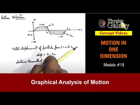
Dear students, now we are going to use graphical analysis of motion. as we are studying rectilinear
motion, in rectilinear motion 3 types of graph are used in motion analysis. we'll see that
these graphs are quite helpful, in solving various kind of problems of, rectilinear
motion also. these three types of graph are. displacement versus time graph. second is,
velocity versus time graph. and the third is, acceleration versus time graph. we also
discuss the variant of displacement time graph as, distance time graph. we'll also discuss
distance versus time graph. we'll also discuss speed versus time graph, because, some particular
type of problems are also asked on distance and speed versus time graphs. but we don't
need to spend much time on these at, slight variations of displacement and velocity time
curves. lets discuss these one by one. now if we talk about displacement versus time
graphs. these are also known as, position versus time graphs. there is no difference
between position versus time and displacement versus time graphs. say for a given rectilinear
motion, we, draw the displacement time curve, like this. so this is the curve, according
to which, the position of a particle varies with time. so its function is given as x=f
of t. in this situation at any instant of time, (t) we can directly get the position
of particle by using, this curve, or by substituting the value of time in this function. say if
this point is p, we draw a tangent , of this curve at this point p, and say it makes an
angle theta with the time axis so we can simply state. the slope of the curve. at point p
can be written as, d x by d t, which is = tan theta. and we all know that d x by d t, can
be directly written as, instantaneous velocity of the particle at this position p. so by,
displacement time graph, at any point if we want to calculate, or we want to evaluate
the instantaneous velocity of the particle, we just need to find out the slope of the
curve, at that point and the slope will be directly give us the, instantaneous velocity
of the particle at that point. so in this situation we can see that, this tangent makes
an acute angle, with the, time axis, here we can simply state the velocity v p which
is tan theta, will be a positive, quantity. if we talk about the decreasing part of the
curve at a point q, if we consider a tangent, you can state, this angle theta dash will
be an obtuse angle. so at point q, the instantaneous velocity can be written as tan theta dash.
and tangent of the obtuse angle can be written as, a negative physical quantity. so in the
decreasing part of curve we can say with time the displacement is coming down, or displacement
is decreasing. or, as if we talk about the position of particle it is moving towards
origin. so we can state vector ally the velocity will be, negative. we can also talk about
various situations, like, for a practical situation. if say, a particle moves, in such
a way, that, first it accelerates, than it moves uniformly, and then say it retards. initially
say it was at rest, and finally also say it'll come to rest. so first it accelerates its
velocity increases, than it moves uniformly, and then finally, it comes to rest. now
in such situations, if particle is accelerating we can simply state the slope will first increase.
and then it moves uniformly that mean its slope remains constant, because you can see
the slope is giving as the instantaneous velocity. and if it it retards, that mean the slope
decreases and finally it becomes zero. so if we draw, the displacement time graph, of
such a motion, we can state first slope is increasing, the curve goes like this you can
see, continual sly the angle which, tangent makes with the time axis increasing. and then
say, for a time t 1 it is, accelerating, and from time t 1 to t 2 or you can say for a
duration t 2, it moves uniformly so we can draw a straight line. so here, the whole slope,
for the duration t 2 remains constant, then it retards, so you can simply draw a curve
like this. which for another duration say t 3. now in this situation finally you can
see the slope become zero and earlier also slope was zero. this is the curve, which
is representing a motion where particle first accelerate, then moves uniformly and then,
retards. similar to this if we just, consider an experimental
situation like, say this positive direction of x axis. from origin a particle starts.
it moves with a velocity v. it goes up to a particular position in a time t 1. then
for a time t 2 it remains at rest over there, and then it comes back to origin, with the
same velocity v. in a time t 3. so from zero to t 1, it was moving uniformly, up to, this
position, say we write maximum displacement x m. for a duration t 2 it remains at rest,
and then, for at time t 2 it'll start, moving in opposite direction, and time t 3 it comes
back. now if we draw, the, position versus time graph, for this motion. you can simply
state it t = 0 particle starts, with an uniform velocity, uniform velocity means the slope
remains constant here we can write tan theta = v. this was the time t 1 for which the particle
was moving uniformly. then you can state up to time t 2, or for the duration t 2 minus
t 1 it remains at rest. so its position remains constant i.e. at, x m. and then, it'll start
coming back so the velocity, is in opposite direction or we can say, when it was moving
toward (right) velocity was positive and now velocity is negative. so it comes down and
at a time t 3 it'll reach the, original position back. so, you can simple state again x becomes
zero. and say this angle is theta dash, so we can again write tan theta dash is equals
to v. now this angle will be, 180 minus theta, and we can state the, tangent of obtuse angle
is negative. so this angle theta dash can be directly taken as the angle by which we
can directly calculate the negative slope. so this is the, curve which is drawn, for
uniform motion then rest for some duration, and then again uniform motion in opposite
direction. now if similar, this is the curve which we call as position time curve or position
time graph. if similar graph is drawn for distance time.
let us draw distance time graph for the same, motion of particle when it is moving then
rest, taking rest and then coming back. so you can simply state, if we talk about displacement,
it first increases to x m then decreases to zero. but when we talk about distance, we
can state distance is continually increasing, because from here to here the distance is
x m, and when it comes back, the total distance travelled by the particle will become 2 x
m. now only difference in position time and distance time graph, can be taken, that, distance
time graph, if this is taken as distance, distance time graph will never come down.
say it'll first increase to a position, of x m, for a time t 1, than, it remains, at
rest, up to a time t 2, and then again it returns back, but if we talk about, position
it is coming down, but if we talk about distance it is still increasing, so the same graph
can be, drawn in reverse direction. so up to a time t 3, it will be able to cover a
distance of 2 x m. this is the distance time graph for the same motion, you can simply
state if we are having a displacement time graph, then for those portions of displacement
time graph, where the curves is coming down, you can draw the mirror image with respect
to time axis in upward direction, that will become, distance time graph.
if we talk about velocity time graphs. these are the graphs relating velocity with time.
say we draw, graph in, velocity and time, for motion of particle, this graph is drawn,
for the function of velocity how it varies with time. at, any position of this graph,
similar to, that of displacement time graph. here if you draw tangent, and you find out
the slope , of this graph, say at point x, we can simply state this point is relating
time with, velocity . and here the slope can be written as d v by d t or it can be written
as tan theta. and here the slope is giving us, the acceleration of particle at the position
x. so always remember that the slope of velocity time graph gives us the, instantaneous acceleration
and, if a slope is positive like, here you can see acceleration at point x, it is
tan theta and theta is acute angle this can be taken as, positive acceleration. positive
acceleration means the velocity, and acceleration have same direction and you can simply state,
the, speed of particle is increasing or the magnitude of velocity is increasing in this
case. when we talk about the decreasing part of the curve, at any position if we draw
tangent, you can see the angle theta dash is obtuse. so this the point y, so we can
say acceleration at point y it'll be tan theta dash, which is an negative quantity. so here
you can see the velocity is decreasing so acceleration we considered to be negative.
so be careful about, the situation, where we have finding the slope of velocity time
curve as, acceleration. along with this we are already studied, in calculus, that area
under a curve can be given by, for between, two, coordinates on time axis, say t 1 and
t 2. if we find out the area of this curve. so area under the curve can be given as,
integration of v d-t from t 1 to t 2 . here you can see, this integration of v d-t, will
be given as displacement only. because, if we talk about v into d-t, it is the displacement
covered by the particle during the time d-t. so if we calculate the total displacement
of particle, from point t 1 to time t 2, it can directly be given as, integration of v
d-t from t 1 to t 2, it'll give us the displacement of particle. from t =, t 1 to, t 2. this
is another advantage of using velocity time graph, that from velocity time graph using
slope we can find out the instantaneous acceleration of particle, and finding out the area under
the curve, like say if we find out this area by using integration, this area under the
curve gives us the, displacement of particle, between two given time instants, in the
given situation.
if we just have a look on motion situation, as shown in the velocity time graph. a particle
moves in such a way that, t= 0 its initial velocity was zero, first velocity increases
that means it was accelerating, and then after some time it'll decreases and again
it become zero at time t 1. than velocity becomes negative, you can say, this is the
negative direction of velocity, and velocity becomes negative that means particle as returned
in opposite direction, and at time t 2 (again) its velocity become zero. so in such situation
you can say from time 0 to t 1. the area between the curve and the time axis, above the time
axis this, positive. and from time t 1 to t 2 you can see, that this area is below the
time axis, so this is written as negative. say, this total area is s1 and this total
area is s 2. so we can state, total displacement. of particle. from t = 0 to t 2. is, total
displacement can be written as s 1 minus s 2. but when we talk about distance travelled.
you can always write distance travelled= s 1 + s 2. because s 1 is the distance travelled,
in positive direction and s 2 is the distance travelled in, opposite direction. so displacement
will be s 1 minus s 2, but when we talk about distance travelled it will be s 1 + s 2, so
be careful about such situations , while drawing velocity time curves. similar to this we can
also talk about, acceleration time graphs. but there is nothing much to discuss about
acceleration time graphs. like if we draw acceleration time graph, for a given motion,
you can simply state in acceleration time graph if we find out the slope. that a slope
will give us the (rate) with which will the acceleration is varying. which is not of much
import ants, in, our limitations, or, in the syllabus we are analyzing the things, but
when we talk about the, (area) under the acceleration time curve or area between the acceleration
time curve and time axis, say between to instants t 1 and t 2, so when it is of, quite importance
like, if we find out this area. this area is say (a) so this (a) can be written as integration
of (a) d-t from time t 1 to t 2. this (a) d-t will give us, net change. in velocity,
of particle. from, t 1 to t 2. there is something which is important for us to keep in mind,
integration of (a) d-t from t1 to t 2 gives us the net change in velocity of particle
in going from, time t 1 to, time t 2. this, you should always keep in mind
Không có nhận xét nào:
Đăng nhận xét